4 Development Tools

Terence Parr and Jeremy Howard

Copyright © 2018-2019 Terence Parr. All rights reserved.
Please don't replicate on web or redistribute in any way.
This book generated from markup+markdown+python+latex source with Bookish.

You can make comments or annotate this page by going to the annotated version of this page. You'll see existing annotated bits highlighted in yellow. They are PUBLICLY VISIBLE. Or, you can send comments, suggestions, or fixes directly to Terence.

Before we dig more into machine learning, let's get familiar with our primary development tools. The code samples in this book explicitly or implicitly use the following important libraries that form the backbone of machine learning with Python for structured data:

• Pandas provides the key data structures we use to hold training and validation sets: data frames and series (columns of data).
• NumPy provides an efficient n-dimensional array data structure used by the other libraries.
• matplotlib provides sophisticated 2D and 3D graphing facilities; Pandas delegates graphing to matplotlib.
• scikit-learn, abbreviated sklearn, has the machine learning models, validation functions, error metrics, and a wide range of data processing facilities.

In the last chapter, we got a taste of using sklearn to train models, and so this chapter we'll focus on the basics of pandas, NumPy, and matplotlib. The development environment we recommend is Jupyter Lab, but you're free to use whatever you're comfortable with. You can skip this chapter if you're itching to get started building models, but it's a good idea to at least scan this chapter to learn what's possible with the libraries before moving on.

4.1 Your machine learning development environment

Over the last 30 years, there's been remarkable progress in the development of IDEs that make programmers very efficient, such as Intellij, Eclipse, VisualStudio, etc... Their focus, however, is on creating and navigating large programs, the opposite of our small machine learning scripts. More importantly, those IDEs have little to no support for interactive programming, but that's exactly what we need to be effective in machine learning. While Terence and Jeremy are strong advocates of IDEs in general, IDEs are less useful in the special circumstances of machine learning.

First, let's make sure that we have the latest version of Jupyter Lab by running this from the Mac/Unix command line or Windows “anaconda prompt” (search for “anaconda prompt” from the Start menu):

The conda program is a packaging system like the usual Python pip tool, but has the advantage that it can also install non-Python files (like C/Fortran code often used by scientific packages for performance reasons.)

Before launching jupyter, it's a good idea to create and jump into a directory where you can keep all of your work for this book. For example, you might do something like this sequence of commands (or the equivalent with your operating system GUI):

On Windows, your user directory is C:\Users\YOURID.

Let's also make a data directory underneath /Users/YOURID/mlbook so that our notebooks can access data files easily:

So that we have some data to play with, download and unzip the data/rent-ideal.csv.zip file into the /Users/YOURID/mlbook/data directory.

Launch the local Jupyter web server that provides the interface by running jupyter lab from the command line:

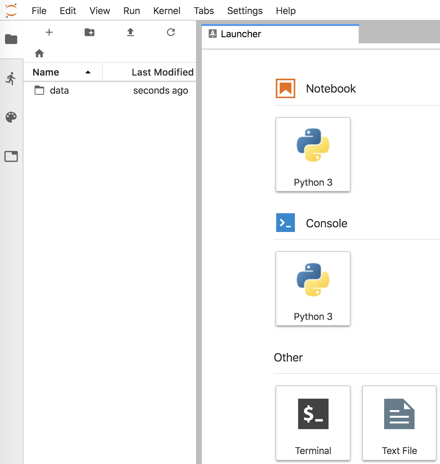
Figure 4.1. Initial Jupyter Lab screen
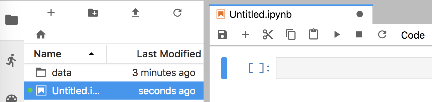
Figure 4.2. Jupyter Lab after creating Python 3 notebook

Running that command should also open a browser window that looks like Figure 4.1. That notebook communicates with the Jupyter Lab server via good old http, the web protocol. Clicking on the “Python 3” icon under the “Notebook” category, will create and open a new notebook window that looks like Figure 4.2. Cut-and-paste the following code into the empty notebook cell, replacing the data file name as appropriate for your directory structure (our set up has file rent-ideal.csv in the mlbook/data subdirectory).

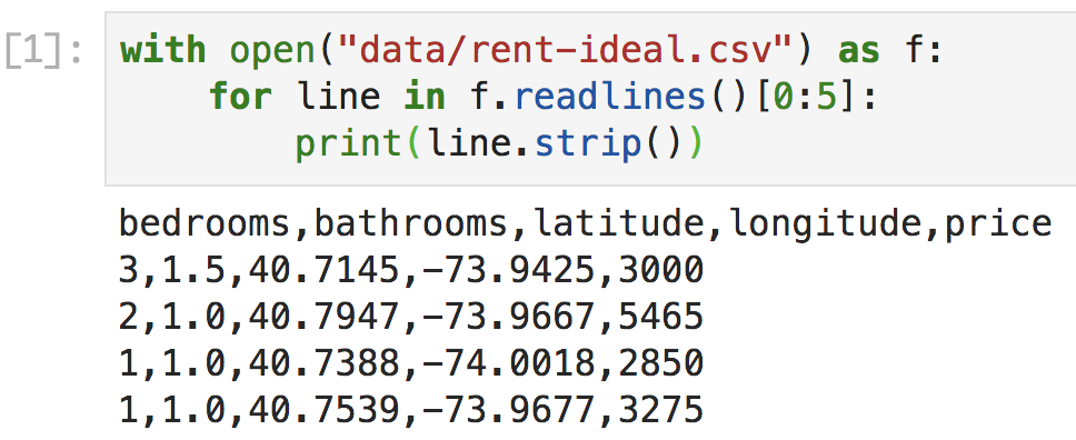
Figure 4.3. Jupyter Lab with one code cell and output

After pasting, hit shift-enter in the cell (hold the shift key and then hit enter), which will execute and display results like Figure 4.3. Of course, this would also work from the usual interactive Python shell:

We could also save that code snippet into a file called dump.py and run it, either from within a Python development environment like PyCharm or from the command line:

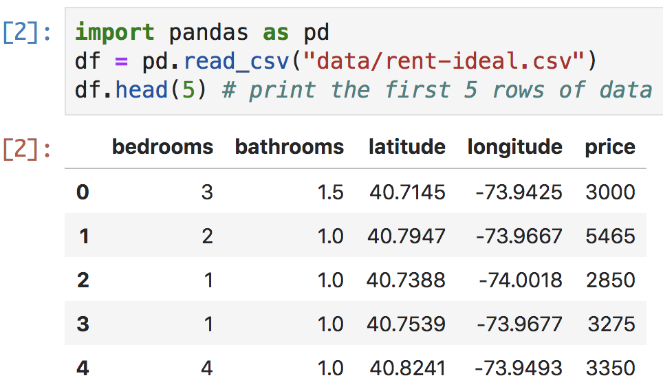
Figure 4.4. Jupyter Lab cell with pandas CSV load
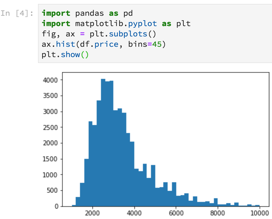
Figure 4.5. Notebook with graph output

Notebooks have some big advantages over the interactive Python shell. Because the Python shell is using an old-school terminal, it has very limited display options whereas notebooks can nicely display tables and even embed graphs inline. For example, Figure 4.4 shows what pandas dataframes look like in Jupyter Lab. Figure 4.5 illustrates how to generate a histogram of rent prices that appears inline right after the code. Click the “+” button on the tab of the notebook to get a new cell (if necessary), paste in the following code, then hit shift-enter.

(We'll learn more about loading dataframes and creating graphs below.)

The Python shell also has the disadvantage that all of the code we type disappears when the shell exits. Notebooks also execute code through Python shells (running within Jupyter Lab's web server), but the notebooks themselves are stored as .ipynb files on the disk. Killing the Python process associated with a notebook does not affect or delete the notebook file. Not only that, when you restart the notebook, all of the output captured during the last run is cached in the notebook file and immediately shown upon Jupyter Lab start up.

Programming with traditional Python .py files means we don't lose our work when Python exits, but we lose interactive programming. Because of its iterative nature, creating and testing machine learning models rely heavily on interactive programming in order to perform lots of little experiments. If loading the data alone takes, say, 5 minutes, we can't restart the entire program for every experiment. We need the ability to iterate quickly. Using a Python debugger from within an IDE does let us examine the results of each step of a program, but the programming part is not interactive; we have to restart the entire program after making changes.

So notebooks combine the important interactive nature of the Python shell with the persistence of files. Because notebooks keep graphics and other output within the document containing the code, it's very easy to see what a program is doing. That's particularly useful for presenting results or continuing someone else's work. You're free to use whatever development environment you find comfortable, of course, but we strongly recommend Jupyter notebooks. If you follow this recommendation, it's a good idea to go through some of the Jupyter tutorials and videos out there to get familiar with your tools.

4.2 Dataframe Dojo

Before we can use the machine learning models in sklearn, we have to load and prepare data, for which we'll use pandas. We recommend that you get a copy of Wes McKinney's book, “Python for Data Analysis,” but this section covers a key subset of pandas functionality to get you started. (You can also check out the notebooks from McKinney's book.) The goal here is to get you started with the basics so that you can get the gist of the examples in this book and can learn more on your own via stackoverflow and other resources.

4.2.1 Loading and examining data

The first step in the machine learning pipeline is to load data of interest. In many cases, the data is in a comma-separated value (CSV) file and pandas has a fast and flexible CSV reader:

The head() method shows the first five records in the data frame, but we can pass an argument to specify the number of records. Data sets with many columns are usually too wide to view on screen without scrolling, which we can overcome by transposing (flipping) the data frame using the T property:

In this way, the columns become rows and wide data frames become tall instead. To get meta-information about the data frame, use method info():

<class 'pandas.core.frame.DataFrame'> RangeIndex: 48300 entries, 0 to 48299 Data columns (total 5 columns): bedrooms 48300 non-null int64 bathrooms 48300 non-null float64 latitude 48300 non-null float64 longitude 48300 non-null float64 price 48300 non-null int64 dtypes: float64(3), int64(2) memory usage: 1.8 MB

It's often useful to get a list of the column names, which we can do easily with a dataframe property:

Index(['bedrooms', 'bathrooms', 'latitude', 'longitude', 'price'], dtype='object')

And, to learn something about the data itself, use describe():

There are also methods to give you a subset of that information, such as the average of each column:

bedrooms 1.508799 bathrooms 1.178313 latitude 40.750782 longitude -73.972365 price 3438.297950 dtype: float64

To get the number of apartments with a specific number of bedrooms, use the value_counts() method:

1 15718 2 14451 0 9436 3 6777 4 1710 5 169 6 36 8 2 7 1 Name: bedrooms, dtype: int64

We can also easily sort a dataframe by a specific column:

4.2.2 Extracting subsets

Preparing data for use in a model often means extracting subsets, such as a subset of the columns or a subset of the rows. Getting a single column of data is particularly convenient in pandas because each of the columns looks like a dataframe object property. For example, here's how to extract the price column from data frame df as a Series object:

<class 'pandas.core.series.Series'> 0 3000 1 5465 2 2850 3 3275 4 3350 Name: price, dtype: int64

df.price is equivalent to the slightly more verbose df['price'], except that df.price does not work on the left-hand side of an assignment when trying to create a new column (see Section 4.2.5 Injecting new dataframe columns).

Once we have a series, there are lots of useful functions we can call, such as the following.

1025 3438.297950310559 9999

If we need more than one column, we can get a dataframe with a subset of the columns (not a list of Series objects):

<class 'pandas.core.frame.DataFrame'>

Data sets typically consist of multiple columns of features and a single column representing the target variable. To separate these for use in training our model, we can explicitly select all future columns or use drop():

The axis=1 bit is a little inconvenient but it specifies we'd like to drop a column and not a row (axis=0). The drop() method does not alter the dataframe; instead it returns a view of the dataframe without the indicated column.

Getting a specific row or a subset of the rows by row number involves using the iloc dataframe property. For example, here's how to get the first row of the dataframe as a Series object:

<class 'pandas.core.series.Series'> bedrooms 3.0000 bathrooms 1.5000 latitude 40.7145 longitude -73.9425 price 3000.0000 Name: 0, dtype: float64

and here's how to get the first two rows as a dataframe:

Those iloc accessors implicitly get all columns, but we can be more explicit with the : slice operator as the second dimension:

bedrooms 3.0000 bathrooms 1.5000 latitude 40.7145 longitude -73.9425 price 3000.0000 Name: 0, dtype: float64

Or, we can use a list of integer indexes to get specific columns:

bedrooms 3.0 price 3000.0 Name: 0, dtype: float64

Generally, though, it's easier to access columns by name by using iloc to get the row of interest and then using dataframe column indexing by name:

bedrooms 3.0 price 3000.0 Name: 0, dtype: float64

4.2.3 Dataframe Indexes

Data frames have indexes that make them behave like dictionaries, where a key maps to one or more rows of a dataframe. By default, the index is the row number, as shown here as the leftmost column:

The loc property performs an index lookup so df.loc[0] gets the row with key 0 (the first row):

bedrooms 3.0000 bathrooms 1.5000 latitude 40.7145 longitude -73.9425 price 3000.0000 Name: 0, dtype: float64

Because the index is the row number by default, iloc and loc give the same result. But we can set index to a column in our dataframe:

Using the index, we can get all 3-bedroom apartments:

Now that the index differs from the default row number index, dfi.loc[3] and dfi.iloc[3] no longer get the same data; dfi.iloc[3] gets 4th row (indexed from 0).

Setting the dataframe index to the bedrooms column means that bedrooms is no longer available as a column, which is inconvenient but a quirk to be aware of: dfi['bedrooms'] gets error KeyError: 'bedrooms'. By resetting the index, bedrooms will reappear as a column and the default row number index will reappear:

Indexing pops up when trying to organize or reduce the data in a data frame. For example, grouping the rows by the values in a particular column makes that column the index. Here's how to group the data by the number of bathrooms and compute the average value of the other columns:

If we want a dataframe that includes bathrooms as a column, we have to reset the indexCan't access bybaths[['bathrooms','price']], must reset first:

and then we can access the columns of interest:

(Notice that the average price for an apartment with no bathroom is $3145. Wow. Evaluating len(df[df.bathrooms==0]) tells us there are 300 apartments with no bathrooms!)

Accessing dataframe rows via the index is essentially performing a query for all rows whose index key matches a specific value, but we can perform much more sophisticated queries.

4.2.4 Dataframe queries

Pandas dataframes are kind of like combined spreadsheets and database tables and this section illustrates some of the basic queries we'll use for cleaning up data sets.

Machine learning models don't usually accept missing values and so we need to deal with any missing values in our data set. The isnull() method is a built-in query that returns true for each missing element in a series:

0 False 1 False 2 False Name: price, dtype: bool

or even an entire dataframe:

Of course, what we really care about is whether any values are missing and any() returns true if there is at least one true value in the series or dataframe:

bedrooms False bathrooms False latitude False longitude False price False dtype: bool

Like a database WHERE clause, pandas supports rich conditional expressions to filter for data of interest. Queries return a series of true and false, according to the results of a conditional expression:

0 False 1 True 2 False 3 True 4 True Name: price, dtype: bool

That boolean series can then be used as an index into the dataframe and the dataframe will return the rows associated with true values. For example, here's how to get all rows whose price is over $3000:

To find a price within a range, we need two comparison operators:

Note that the parentheses are required around the comparison subexpressions to override the high precedence of the & operator. (Without the parentheses, Python would try to evaluate 1000 & df.price.)

Compound queries can reference multiple columns. For example here's how to get all apartments with at least two bedrooms that are less than $3000:

4.2.5 Injecting new dataframe columns

After selecting features (columns) and cleaning up a data set using queries, data science practitioners often create new columns of data in an effort to improve model performance. Creating a new column with pandas is easy, just assign a value to the new column name. Here's how to make a copy of the original df and then create a column of all zeroes in the new dataframe:

That example just shows the basic mechanism; we'd rarely find it useful to set a column of zeros. On the other hand, we might want a column of random numbers to see how it affected model performance. Here's how to overwrite the junk column using a NumPy array of random numbers:

A word of warning when injecting new columns into a dataframe subset. Injecting a new column into, say, df is no problem as long as df is the entire data frame, and not a subset (sometimes called a view). For example, in the following code, bedsprices is a subset of the original df; pandas returns of view of the data rather than inefficiently creating a copy.

Trying to inject a new column yields a warning from pandas:

Essentially, pandas does not know whether we intend to alter the original df or to make bedsprices into a copy and alter it but not df. The safest route is to explicitly make a copy:

See Returning a view versus a copy from the pandas documentation for more details.

4.2.6 String and date operations

Dataframes have string and date-related functions that are useful when deriving new columns or cleaning up existing columns. To demonstrate these, we'll need a data set with more columns, so download and unzip rent.csv.zip into your mlbook/data directory. Then use read_csv to load the rent.csv file and display five columns:

The parse_dates parameter make sure that the created column is parsed as a date not a string. Column features is a string column (pandas labels them as type object) whose values are comma-separated lists of features enclosed in square brackets, just as Python would display a list of strings. Here's the type information for all columns in rent.csv:

<class 'pandas.core.frame.DataFrame'> RangeIndex: 49352 entries, 0 to 49351 Data columns (total 5 columns): created 49352 non-null datetime64[ns] features 49352 non-null object bedrooms 49352 non-null int64 bathrooms 49352 non-null float64 price 49352 non-null int64 dtypes: datetime64[ns](1), float64(1), int64(2), object(1) memory usage: 1.9+ MB

The string-related methods are available via series.str.method(); the str object just groups the methods. For example, it's a good idea to normalize features of string type so that doorman and Doorman are treated as the same word:

As part of the normalization process, it's a good idea to replace any missing values with a blank and any empty features column values, [], with a blank:

Pandas uses “not a number”, NumPy's np.nan, as a placeholder for unavailable values, even for nonnumeric string and date columns. Because np.nan is a floating-point number, a missing integer flips the entire column to have type float. See Working with missing data for more details.

Looking at the string values in the features column, there is a good deal of information that would potentially improve the model's performance. Models would not generally be able to automatically extract useful features and so we have to give them a hand. The following code creates two new columns that indicates whether or not the apartment has a doorman or laundry ("laundry|washer" is a regular expression that matches if either laundry or washer is present).

Ultimately, models can only use numeric or boolean data columns, so these conversions are very common. Once we've extracted all useful information from the raw string column, we would typically delete that features column.

Instead of creating new columns, sometimes we convert string columns to numeric columns. For example, the interest_level column in the rent.csv data set is one of three strings (low, medium, and high):

type of interest_level is object

An easy way to convert that to a numeric column is to map each string to a unique value:

type of interest_level is int64

For large data sets, sometimes it's useful to reduce numeric values to the smallest entity that will hold all values. In this case, the interest_level values all fit easily within one byte (8 bits), which means we can save a bunch of space if we convert the column to int8 from int64:

type of interest_level is int8

Like string columns, models cannot directly use date columns, but we can break up the date into a number of components and derive new information about that date. For example, imagine training a model that predicts sales at a grocery market. The day of the week, or even the day of the month, could be predictive of sales. People tend to shop more on Saturday and Sunday than during the week and perhaps more shopping occurs on monthly paydays. Maybe there are more sales during certain months like December (during Christmas time). Pandas provides convenience methods, grouped in property dt, for extracting various date attributes and we can use these to derive new model features:

Once we've extracted all useful numeric data, we'd drop column created before training our model on the data set.

4.2.7 Merging dataframes

Imagine we have a df_sales data frame with lots of features about sales transactions, but let's simplified to just two columns for discussion purposes. The problem we have is that price information is in a different dataframe, possibly because we extracted the data from a different source. The two dataframes look like the following.

Our goal is to create a new column in df_sales that has the appropriate SalePrice for each record. To do that, we need a key that is common to both tables, which is the SalesID in this case. For example, the record in df_sales with SalesID of 1222843 should get a new SalesPrice entry of 10000. In database terms, we need a left join, which keeps all records from the left dataframe and ignores records for unmatched SalesIDs from the right dataframe:

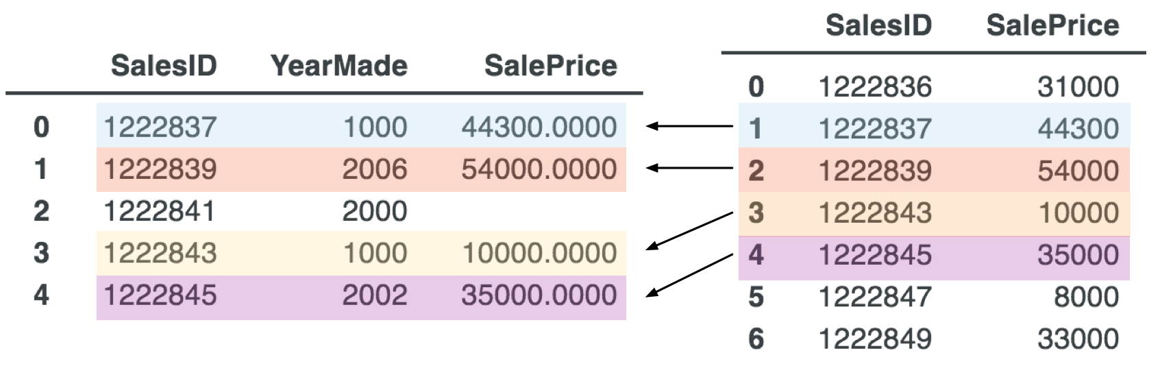
Any record in the left dataframe without a counterpart in right dataframe gets np.NaN (not a number) to represent a missing entry.

In Python the merge operation looks like:

The left join makes a bit more sense sometimes when we see the right join. A right join keeps all records in the right dataframe, filling in record values for unmatched keys with np.NaN:

4.2.8 Saving and loading data in the feather format

Data files are often in CSV, because it is a universal format and can be read by any programming language. But, loading CSV files into dataframes is not very efficient, which is a problem for large data sets during the highly iterative development process of machine learning models. The author of pandas, Wes McKinney, and Hadley Wickham (a well-known statistician and R programmer) recently developed a new format called feather that loads large data files much faster than CSV files. Given a dataframe, here's how to save it as a feather file and read it back in:

We performed a quick experiment, mirroring the one done by McKinney and Wickham in their original blog post from 2016. Given a data frame with 10 columns each with 10,000,000 floating-point numbers, pandas takes about two minutes to write it out as CSV to a fast SSD drive. In contrast, it only takes 1.5 seconds to write out the equivalent feather file. Also, the CSV file is 1.8G versus only 800M for the feather file. Reading the CSV file takes 22s versus 6s for the feather file. Here is the test rig, adapted from McKinney and Wickham:

Now that we know how load, save, and manipulate dataframes, let's explore the basics of visualizing dataFrame data.

4.3 Generating plots with matplotlib

Matplotlib is a free and widely-used Python plotting library. There are lots of other options, but matplotlib is so well supported, it's hard to consider using anything else. For example, there are currently 34,515 matplotlib questions on stackoverflow. That said, we find it a bit quirky and the learning curve is pretty steep. Getting basic plots working is no problem, but highly-customized plots require lots of digging in the documentation and with web searches. The goal of this section is to show how create the three most common plots: scatter, line, and histogram.

Each matplotlib plot is represented by a Figure object, which is just the drawing surface. The graphs or charts we draw in a figure are called Axes (a questionable name due to similarity with “axis”) but it's best to think of axes as subplots. Each figure has one or more subplots. Here is the basic template for creating a plot:

Let's use that template to create a scatterplot using the average apartment price for each number of bedrooms. First, we group the rent data in df by the number of bedrooms and ask for the average (mean). To plot bedrooms versus price, we use the scatter method of the ax subplot object:

» Generated by code to left

bybeds = df.groupby(['bedrooms']).mean() bybeds = bybeds.reset_index() # make bedrooms column again fig, ax = plt.subplots() ax.scatter(bybeds.bedrooms, bybeds.price, color='#4575b4') ax.set_xlabel("Bedrooms") ax.set_ylabel("Price") plt.show()

With some self explanatory methods, such as set_xlabel(), we can also set the X and Y axis labels. Drawing a line in between the points, instead of just a scatterplot, is done using method plot():

» Generated by code to left

fig, ax = plt.subplots() ax.plot(bybeds.bedrooms, bybeds.price, color='#4575b4') ax.set_xlabel("Bedrooms") ax.set_ylabel("Price") plt.show()

If we have a function to plot over some range, instead of data, we can still use plot(). The function provides the Y values, but we need to provide the X values. For example, let's say we'd like to plot the log (base 10) function over the range 0.01 to 100. To make it smooth, we should evaluate the log function at, say, 1000 points; NumPy's linspace() works well to create the X values. Here's the code to make the plot and label the axes:

» Generated by code to left

x = np.linspace(0.01, 100, 1000) y = np.log10(x) # apply log10 to each x value fig, ax = plt.subplots() ax.plot(x, y, color='#4575b4') plt.ylabel('y = log_base_10(x)') plt.xlabel('x') plt.show()

Creating a histogram from a dataFrame column is straightforward using the hist() method:

» Generated by code to left

fig, ax = plt.subplots() ax.hist(df.price, color='#4575b4', bins=50) ax.set_xlabel("Price") ax.set_ylabel("Count of apts") plt.show()

Such plots approximate the distribution of a variable and histograms are a very useful way to visualize columns with lots of data points. Here, we see that the average price is roughly $3000 and that there is a long “right tail” (with a few very expensive apartments).

The last trick we'll consider here is getting more than one plot into the same figure. Let's take two of the previous graphs and put them side-by-side into a single figure. The code to generate the individual graphs is the same, except for the Axes object we use for plotting. Using the subplots() method, we can specify how many rows and columns of subplots we want, as well as the width and height (in inches) of the figure:

For some reason, matplotlib does not automatically adjust the space between subplots and so we generally have to call plt.tight_layout(), which tries to adjust the padding. Without that call, the plots overlap.

There's one more library that you will encounter frequently in data science code, and that is Numpy. We've already used it for such things as creating random numbers and representing “not a number” (np.nan).

4.4 Representing and processing data with NumPy

Pandas dataframes are meant to represent tabular data with heterogeneous types, such as strings, dates, and numbers. NumPy, on the other hand, is meant for performing mathematics on n-dimensional arrays of numbers. (See NumPy quickstart.) The boundaries between pandas, matplotlib, NumPy, and sklearn are blurred because they have excellent interoperability. We can create dataframes from NumPy arrays and we can get arrays from pandas dataframes. Matplotlib and sklearn functions accept both pandas and NumPy objects, automatically doing any necessary conversions between datatypes.

The fundamental data type in NumPy is the np.ndarray, which is an n-dimensional array data structure. A 1D ndarray is just a vector that looks just like a list of numbers. A 2D ndarray is a matrix that looks like a list of lists of numbers. Naturally, a 3D ndarray is a rectangular volume of numbers (list of matrices), and so on. The underlying implementation is highly optimized C code and NumPy operations are much faster than doing the equivalent loops in Python code. The downside is that we have yet more library functions and objects to learn about and remember.

Let's start by creating a one dimensional vector of numbers. While the underlying data structure is of type ndarray, the constructor is array():

type is <class 'numpy.ndarray'> dtype is int64 ndim is 1 [1 2 3 4 5]

By default, the array has 64-bit integers, but we can use smaller integers if we want:

int8 [1 2 3 4 5]

To initialize a vector of zeros, we call zeros with a tuple or list representing the shape of the array we want. In this case, let's say we want five integer zeros:

[0 0 0 0 0]

Similarly, here's how to initialize an array with ones:

[1. 1. 1. 1. 1.]

The equivalent to Python's range function is arange():

[ 1 2 3 4 5 6 7 8 9 10]

When creating a sequence of evenly spaced floating-point numbers, use linspace (as we did above to create values between 0.1 and 100 to plot the log function). Here's how to create 6 values from 1 to 2, inclusively:

[1. 1.2 1.4 1.6 1.8 2. ]

Using raw Python, we can add two lists of numbers together to get a third very easily, but for long lists speed could be an issue. Delegating vector addition, multiplication, and other arithmetic operators to NumPy gives a massive performance boost. Besides, data scientists need to get use to doing arithmetic with vectors (and matrices) instead of atomic numbers. Here are a few common vector operations performed on 1D arrays:

[1 2 3 4 5] + [1 2 3 4 5] = [ 2 4 6 8 10] [1 2 3 4 5] - [1. 1. 1. 1. 1.] = [0. 1. 2. 3. 4.] [1 2 3 4 5] * [0 0 0 0 0] = [0 0 0 0 0] np.dot([1 2 3 4 5], [1 2 3 4 5]) = 55

Aside from the arithmetic operators, there are lots of common mathematical functions we can apply directly to arrays without resorting to Python loops:

[1.09861229 1.94591015 2.19722458 2.19722458 0.69314718] 6.0 9 30

The expression np.log(prices) is equivalent to the following loop and array constructor, but the loop is much slower:

We ran a simple test to compare the speed of np.log(prices) on 50M random numbers versus np.log on a single number via the Python loop. NumPy takes half a second but the Python loop takes over a minute. That's why it's important to learn how to use these libraries, because using straightforward loops is usually too slow for big data sets.

Now, let's move on to matrices, two dimensional arrays. Using the same array() constructor, we can pass in a list of lists of numbers. Here is the code to create two 4 row x 5 column matrices, t and u, and print out information about matrix t:

type is <class 'numpy.ndarray'> dtype is int64 ndim is 2 shape is (4, 5) [[1 1 1 1 1] [0 0 1 0 0] [0 0 1 0 0] [0 0 1 0 0]]

As another example of matplotlib, let's treat those matrice as two-dimensional images and display them using method imshow() (image show):

» Generated by code to left

fig, axes = plt.subplots(1,2,figsize=(2,1)) # 1 row, 2 columns axes[0].axis('off') axes[1].axis('off') axes[0].imshow(t, cmap='binary') axes[1].imshow(u, cmap='binary') plt.show()

There are also built-in functions to create matrices of zeros:

[[0. 0. 0. 0.] [0. 0. 0. 0.] [0. 0. 0. 0.]]

and random numbers, among others:

[[0.51437402 0.46566841 0.20536907] [0.82139522 0.11044102 0.66979215]]

Indexing 1D NumPy arrays works like Python array indexing with integer indexes and slicing, but NumPy arrays also support queries and list of indices, as we'll seen shortly. Here are some examples of 1D indexing:

[1 2 3 4 5] 1 5 [2 3] [3 5]

For matrices, NumPy indexing is very similar to pandas iloc indexing. Here are some examples:

[1 1 1 1 1] [1 1 1 1] 0 [[1 1 1 1 1] [0 0 1 0 0]] [[1 1] [0 1] [0 1] [0 1]]

As with pandas, we can perform queries to filter NumPy arrays. The comparison operators return a list of boolean values, one for each element of the array:

[0.63507935 0.51535146 0.34574814 0.38985047 0.92781766] [ True True True True True]

We can then use that array of booleans to index into that array, or even another array of the same length:

[1 2 3 4 5]

As with one dimensional arrays, vectors, the NumPy defines the arithmetic operators for matrices. For example, here's how to add and print out two matrices:

[[2 1 1 1 2] [1 0 1 0 1] [1 0 1 0 1] [1 1 2 1 1]]

If we make an array of matrices, we get a 3D array:

type is <class 'numpy.ndarray'> dtype is int64 ndim is 3 [[[1 1 1 1 1] [0 0 1 0 0] [0 0 1 0 0] [0 0 1 0 0]] [[1 0 0 0 1] [1 0 0 0 1] [1 0 0 0 1] [1 1 1 1 1]]]

Sometimes, we'd like to go the opposite direction and unravel (ravel is a synonym) flatten a multidimensional array. Imagine we'd like to process every element of the matrix. We could use nested loops that iterated over the rows and columns, but it's easier to use a single loop over a flattened, 1D version of the matrix. For example, here is how to sum up the elements of matrix u:

11

The flat property is an iterator that is more space efficient than iterating over u.ravel(), which is an actual 1D array of the matrix elements. If you don't need a physical list, just iterate using the flat iterator.

11 [1 0 0 0 1 1 0 0 0 1 1 0 0 0 1 1 1 1 1 1]

To iterate through the rows of a matrix instead of the individual elements, use the matrix itself as an iterator:

0: [1 1 1 1 1] 1: [0 0 1 0 0] 2: [0 0 1 0 0] 3: [0 0 1 0 0]

NumPy has a general method for reshaping n-dimensional arrays. The arguments of the method indicate the number of dimensions and how many elements there are in each dimension.

4x3 [[ 1 2 3] [ 4 5 6] [ 7 8 9] [10 11 12]] 3x4 [[ 1 2 3 4] [ 5 6 7 8] [ 9 10 11 12]] 2x6 [[ 1 2 3 4 5 6] [ 7 8 9 10 11 12]]

One of the dimension arguments can be -1, which is kind of a wildcard. Given the total number of values in the array and n-1 dimensions, NumPy can't figure out the dimension. It's very convenient when we know how many rows or how many columns we want because we don't have to compute the other dimension size. Here's how to create a matrix with 4 rows and a matrix with 2 columns using the same data:

4x? [[ 1 2 3] [ 4 5 6] [ 7 8 9] [10 11 12]] ?x2 [[ 1 2] [ 3 4] [ 5 6] [ 7 8] [ 9 10] [11 12]]

The reshape method comes in handy when we'd like to run a single test vector through a machine learning model. Let's train a random forest regressor model on the rent-idea.csv data using price as the target variable:

And, here's a test vector describing an apartment for which we'd like a predicted price. The sklearn predict() method is expecting a matrix of test vectors, rather than a single test vector.

If we try sending the test vector in, rf.predict(test_vector), we get error:

There's a big difference between a 1D vector and 2D matrix with one row (or column). Since sklearn is expecting a matrix, we need to send in a matrix with a single row and we can conveniently convert the test vector into a matrix with one row using reshape(1,-1):

[[ 2. 1. 40.7947 -73.9957]] -> [4873.48418398]

Notice that we also get a vector of predictions (with one element) back because predict() is designed to map multiple test vectors to multiple predictions.

Let's finish up our discussion of NumPy by looking at how to extract NumPy arrays from pandas dataframes. Given a dataframe or column, use the values dataframe property to obtain the data in a NumPy array. Here are some examples using the rent data in df:

[3000 5465 2850 ... 2595 3350 2200]

[ 3.00000e+00 1.50000e+00 4.07145e+01 -7.39425e+01 3.00000e+03]

[[3. 1.5] [2. 1. ] [1. 1. ] ... [1. 1. ] [0. 1. ] [2. 1. ]]

That wraps up our whirlwind tour of the key libraries, pandas, matplotlib, and NumPy. Let's apply them to some machine learning problems. In the next chapter, we're going to re-examine the apartment data set used in Chapter 3 A First Taste of Applied Machine Learning to train a regressor model, but this time using the original data set. The original data has a number of issues that prevent us from immediately using it to train a model and get good results. We have to explore the data and do some preprocessing before training a model.