2 How Machine Learning Works

Terence Parr and Jeremy Howard

Copyright © 2018-2019 Terence Parr. All rights reserved.
Please don't replicate on web or redistribute in any way.
This book generated from markup+markdown+python+latex source with Bookish.

You can make comments or annotate this page by going to the annotated version of this page. You'll see existing annotated bits highlighted in yellow. They are PUBLICLY VISIBLE. Or, you can send comments, suggestions, or fixes directly to Terence.

“Without data you're just another person with an opinion” — W. Edwards Deming

In densely-populated cities, such as San Francisco and New York, everyone's favorite topic is the cost of housing. There's nothing quite as invigorating as writing a check for US$4200/month to rent a single bedroom apartment (as renters do down the street from Terence's place in San Francisco's Mission District). People are always comparing rent prices because they want to know if they're overpaying or getting a good deal. The idea is to collect information on similar apartments and then compare prices. Real estate agents tend to have more data and are, hopefully, able to provide more accurate rent estimates.

The goal of this chapter is to get an idea of how machine learning works. To do that, let's try to invent a technique for predicting apartment rent prices in New York City. It'll highlight the difficulty of the problem and help us understand the machine learning approach. Without understanding the underlying algorithms, we can't successfully apply machine learning. We must be able to choose the right algorithm for a particular problem and be able to properly prepare data for that algorithm. By starting simply and going down a few dead ends, we'll also motivate the construction of more sophisticated techniques. Along the way, we'll define a number of important terms and concepts commonly used by machine learning practitioners and give a general overview of the machine learning process.

2.1 Learning to Learn about Apartment Data

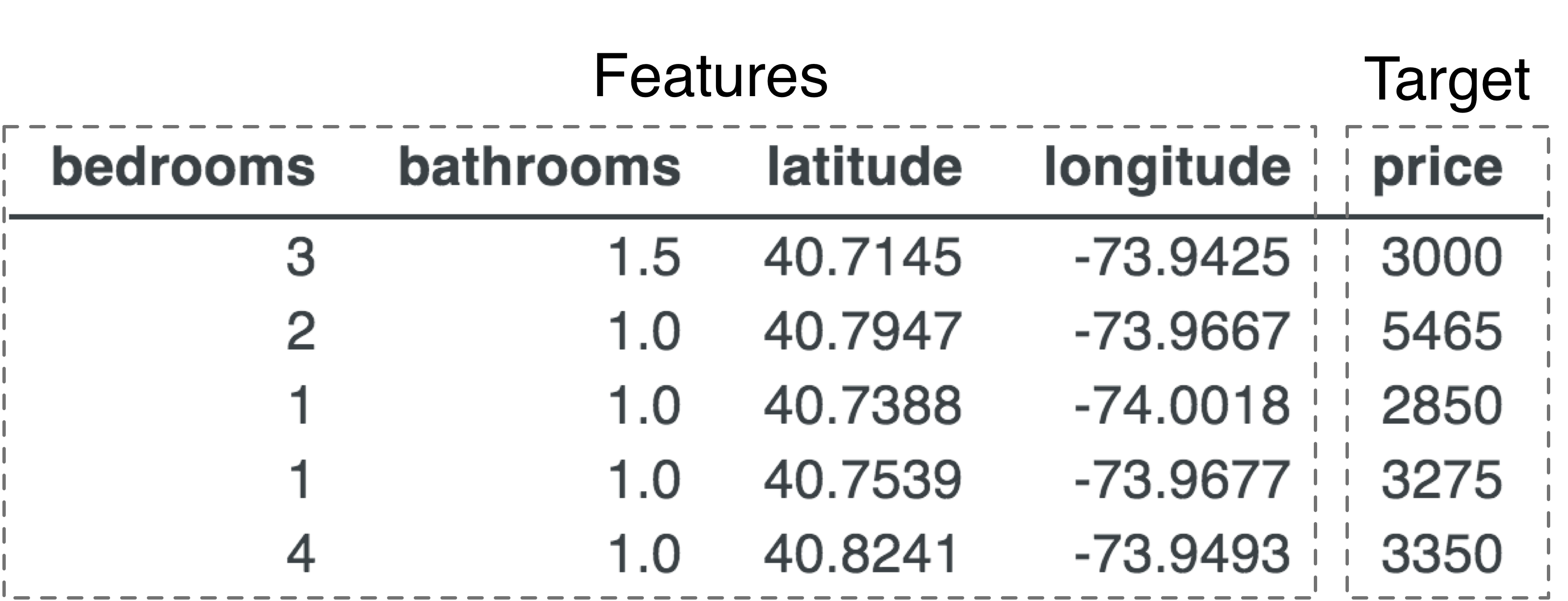
As with any problem-solving exercise, it's a good idea to start by clearly defining the problem. Given four attributes of an apartment, the number of bedrooms, the number of bathrooms, and location (longitude, latitude) we want to predict (determine) the price. Those apartment attributes are called features and the price is called the target. We're usually given data in the form of a table like the following.

This data is called training data or the training set because we, or a program, must learn from this “experience” in order to make predictions. (It's often convenient to treat all of the features for a single record as a single feature vector; a vector is a list of numbers.)

The central problem of machine learning is to build a system that is accurate without being overly-specific to this training data (assuming the data has an underlying relationship to capture).

It's easy to build a system that makes accurate predictions for items in the training set. All we have to do is memorize the apartments and their prices (in this context) then look up the price for an apartment in the training data when asked to do so. At the other extreme, we could compute the average rent across all apartments and predict that price for any apartment look up, inside or outside of the training data. The overall average rent would not be super accurate for a specific apartment, but it would give a ballpark figure, easily distinguishing rent from, say, a hot pastrami sandwich at Katz's delicatessen on E. Houston Street ($21.45).

Memorization doesn't generalize beyond the training data but is precise. Blurring all apartments together obviously yields a prediction for any apartment we present but is not precise at all. Somewhere in between lies effective machine learning. Let's start with just memorizing the training data and work our way towards a system that properly generalizes.

2.1.1 Learning by rote

Given the training data, we can reasonably predict a price of $5,465 for an apartment with two bedrooms and one bathroom at location coordinates 40.7947,-73.9667 because that comes straight from the second row of the table. To get perfect accuracy, we can interpret the learning process conceptually as just filling up a dictionary that maps a four-element key to a single value (price), something like this:

In the vocabulary of machine learning, we are “training a model,” where the model here is a dictionary data structure. Training in this case simply means to remember all apartment data with perfect recall.

But this training process assumes that all apartment records are unique, which is not a valid assumption. For example, here are four studio apartments with the same (bedrooms, bathrooms, latitude, longitude) feature vector but different (eye-popping!) prices:

Having multiple prices for the same feature vector represents an uncertainty. Which of the four prices should the model return? There's likely a good reason for the difference in prices, such as view or square footage, but we don't have that data. Or, as we'll see in Chapter 5 Exploring and Denoising Your Data Set, data is sometimes noisy or just plain wrong. Either way, we need to deal with this uncertainty because repeated keys cause our rudimentary training process to overwrite previous prices.

Because our goal is to generalize, giving a good estimate for apartments not in our training data, we should aim for the expected rent value considering all apartments in the city with the same attributes. Another term for expected value is “average” so let's just record the average, which is what a human expert would do implicitly. In this case, we'd record an average price ($2,825) and yield that value when asked to predict the price of an apartment with those features. The more sample prices in our training data we have for a particular set of apartment attributes, the better the estimate of the true average price we'd get. This works well and is actually a kind of lossy compression because we have merged records, at the cost of less specific predictions.

Aggregating records for identical apartment feature vectors and recording their average rent dips a toe into the as-yet murky waters of machine learning. We are creating an aggregate price for a prototypical apartment of a particular type, in a sense learning what the price should be or is expected to be for that type of apartment. This gives us a hint that machine learning is a just a sensible combination of data structures, algorithms, and statistics. As we continue, hopefully you'll see that machine learning is not some mysterious and arcane mechanism that takes forever to learn.

2.1.2 Getting to know the neighbors

The problem with the rudimentary dictionary model is that it's super rigid in that it can't deal with uncertainty in the apartment feature vectors themselves. (Previously-unseen apartment feature combinations raise a “key error” during look up.) How should we predict the price of an apartment whose features don't exactly match an entry in the training data?

An interesting solution is to keep the original training data as-is and then scan for the apartment record whose features most closely match the features of the apartment for which we'd like a price. As before, there could be multiple prices for that closest matching record and so we'd want to average those prices to yield the prediction. Believe it or not, such a simple model is very powerful (for appropriate data sets) and is a variation on what's called a k nearest neighbor predictor (See kNN).

The only problem with the nearest neighbor model is performance. We have to keep the entire training data set around as the model and we have to linearly scan all of the records looking for the closest match for an apartment feature vector. In contrast to the dictionary model, there is no training process, but apartment lookup (prediction) is very slow.

Another way to handle uncertainty in the apartment features, is to merge records as we did before. We can group apartment records by a combination of bedrooms and bathrooms and compute the average price for each group. This approach works in this case because there are only so many combinations of numbers of bedrooms and bathrooms; we can cover them all. For example, here are the first few average prices per bedrooms/bathrooms combination:

(You gotta like New York City and its quirky apartments; apparently you can rent places with no bedroom but 4 bathrooms for an average of $7995/month!)

At the cost of specificity, merging dramatically reduces the size of the data set, from 48,266 records down to 51 records for this data set. A dictionary or linear scan could quickly find the bedrooms/bathrooms combination to make a prediction. Of course, this approach completely ignores location, which we know to be important. The group averages are hiding a lot of variability between apartments. We could make a secondary index that grouped apartments by latitude/longitude to get a second estimate based solely on the location. But it's unclear how we would merge the two rent estimates into a single prediction. Such an ad hoc approach sometimes works but requires a lot of thought and is highly dependent upon the data set. We need a more systematic approach.

2.1.3 Drawing the line

We could try a “mathy” approach where we weight each feature by how important it is then use a weighted sum to estimate rent prices:

This equation boils all of our rent training data down to just five numbers that comprise our model (four weights, w_i, and a scalar for minimum rent). That's an amazing compression! Better yet, making a prediction is superfast because it's just four multiplies and four additions.

This approach often works well and is called a linear model or linear regression because it tries to draw a line (or plane when given more than two dimensions) through the training data. (Recall the formula for a line from high school algebra, .) The technique has been around for over 200 years and mathematicians have an elegant formula to conjure up suitable w_i weights. Regression is the general term for predicting numerical values based upon training data and the associated model is called a regressor.

Figure 2.1. Price per number of bathrooms and linear regression fit line

For this data set, unfortunately, a linear model is not a good choice because such models treat every feature as a single trend with lower rent on one side and higher rent on the other, or vice versa. For example, it's reasonable to assume that rent prices would go up as the number of bathrooms goes up, but the data doesn't support that conclusion. Figure 2.1 shows the average rent for all apartments with the same number of bathrooms with dots where we actually have data.

The “best fit,” red line minimizes the difference between the line and the actual average price but is clearly a terrible predictor of price. In this case, there is something weird going on beyond 4 bathrooms. (10 bathrooms and only $3500/month? One can only imagine what those places look like.) Consequently, a single line is a poor fit and does not capture jagged relationships like this very well.

2.1.4 Walking through the trees

A more sophisticated approach would treat different ranges of a feature's values separately, giving a different rent estimate per range. Each feature range would have a different prototypical apartment. But, we have to be careful not to create a model that is too specific to the training data because it won't generalize well. We don't want to go lurching back to the other extreme, towards a dictionary model that memorizes exact apartment feature vector to price relationships.

We want a model that gracefully throttles up, splitting a feature's values into as many ranges as necessary to get decent accuracy but without creating so many tight ranges it kills generality. To see how such a model might work, let's consider the rent prices for one-bath, one- and two-bedroom apartments in a very small rectangular region of New York:

An easy but tedious way to capture the relationship between the feature values and the associated price would be to define some rules in Python:

With enough coffee, we should be able to come up with the rules to carve up the feature space (4-dimensional space of all possible bedrooms, bathrooms, latitude, longitude combinations) into clusters. Ideally, each cluster would contain apartments with similar attributes and similar rent, as is the case for this subsample. To make a rent prediction, we'd execute the rules until we get a match for the apartment features of interest.

Unlike the dictionary model, these rules can handle previously unseen data. For example, imagine a one-bedroom, one-bathroom apartment at location 40.6612,-73.9800 that does not exist in the training data. The first rule applies and so the model would predict rent of $2,143. This model generalizes (at least somewhat) because it deals in ranges of feature values not exact feature values.

The size and number of feature value ranges used by the model represent a kind of an accuracy “knob.” Turning the knob one way increases generality but makes the model potentially less accurate. In the opposite direction, we can make the ranges tighter and the model more accurate, but we potentially lose generality. A model that is overly-specific to the training data and not general enough is said to overfit the training data. The opposite, naturally, is an underfit model that doesn't capture the relationships in the training data well, which also means that it won't generalize well.

Okay, now we have a model that is potentially accurate and general but prediction through sequential execution of numerous if-statements would be pretty slow. The trick to making prediction efficient is to factor and nest the rules so they share comparisons to avoid repeated testing:

Figure 2.2. Sample partial regressor decision tree

Another way to encode those nested rules is with a tree data structure, where each node performs a comparison. Figure 2.2 is a visual representation of what such a tree might look like. Predicting rent using such a tree costs just four comparisons as we descend from root to the appropriate leaf, testing features as we go. The leaves of the tree contain the prices for all apartments fitting the criteria on the path from the root down to that leaf. Trees like this are called decision trees and, if we allow the same feature to be tested multiple times, decision trees can carve up feature spaces into arbitrarily tight clusters.

The problem with decision trees is that they tend to get too specific; they overfit training data. For example, we could build a decision tree that carved up the feature space so that each leaf corresponded to a single apartment. That'd provide precise answers but, as with our rudimentary dictionary model, such a specific tree would not generalize.

2.2 Random Forest Regressors

To prevent overfitting, we can weaken the decision tree by reducing its accuracy in a very specific way: By training the tree on a random selection of the training data instead of all members of the data set. (Technically, we are bootstrapping, which randomly selects records but with replacement, meaning that a record can appear multiple times in the bootstrapped sample.) To reduce overfitting even further, we can sometimes forget that certain features exist, such as the number of bedrooms. Because not all elements from the original data set are present, we have a coarser view of the training data so the comparison ranges in our decision tree nodes will necessarily be broader.

To compensate for this weak learner, we can create lots of them and take the average of their individual predictions to make an overall rent prediction. We call this ensemble learning and it's an excellent general technique to increase accuracy without such a strong tendency to overfit. Introducing more randomness gives us a Random Forest™, which we'll abbreviate as RF.

An RF behaves very much like a group of real estate agents looking for comparable apartments and cooperating to estimate an apartment's price (“crowdsourcing”). In the training process the agents would independently select and visit available apartments in New York City. The selection of apartments should be random to reduce the possibility that an agent only visits, say, one-bedroom apartments. Such an agent would be “overfit” in the sense that they could only give reasonable answers for one bedrooms. Randomly selecting apartments reduces the possibility of such sampling bias. Each agent would train on a different sample of apartments but with some overlap. Adding more agents improves our prediction accuracy and model generality, without increasing the probability of overfitting.

To predict the price of an apartment with a particular set of features, each agent would find comparable (similar or identical) apartments from their training set and report the average of those apartments. The overall prediction would then be the average of all agents' averages.

We'll learn the details of random forests in Chapter 17 Forests of Randomized Decision Trees and how to implement them in Chapter 18 Implementing Random Forests. RFs are the Swiss Army Knife™ of the machine learning world and we recommend them as your model of choice for the majority of machine learning problems encountered in practice.

With a small tweak, we can use random forests for a related and equally-useful task: predicting discrete categories like cancer/not-cancer instead of continuous values such as prices.

2.3 Random Forest Classifiers

We've all been to the doctor to present a set of symptoms and ask for a diagnosis. We'd like to know whether that rash is poison ivy, an abrasion, a virus, or skin cancer. In response, the doctor provides a diagnosis consisting of the name of the disease or condition. Or, we might simply want to know whether our symptoms are something to worry about, in which case the doctor provides a binary yes/no answer. A machine learning model providing such a diagnosis is called a classifier because it predicts a class or category (disease name) rather than predicting a numeric value like rent price.

Doctors implicitly compute disease likelihoods from their experience in order to make a diagnosis. Roughly speaking, a doctor analyzes the situation by thinking: “I've seen similar symptoms 10 times; 7 of those people had disease A, 2 had disease B, and 1 had disease C.” The diagnosis is then disease A if we apply a decision rule that picks the disease with the most “votes” (highest likelihood). That sounds just like the nearest neighbor (kNN) approach we used in Section 2.1.2 Getting to know the neighbors to predict rent prices.

A kNN classifier finds k similar patient case histories, per the feature vectors of symptoms, and takes a majority diagnosis “vote” among those k. The only difference between a kNN regressor and classifier is that the regressor yields the average of the target values for the k similar records and a kNN classifier yields the target category that is in the majority among the k similar records.

In the abstract, decision trees are carving up the feature space into groups of similar observations just like kNN models do. Each leaf represents one of these groups. The difference between regressors and classifiers is that leaves in regressor trees predict numeric values while leaves in classifier trees predict discrete categories. A regressor leaf predicts the average of the target values from the observations grouped in that leaf and a classifier leaf predicts the most common target category. An RF classifier is just an ensemble of classifier decision trees that yields the most likely category predicted among the trees. In that sense, it's kind of a meta-voting scheme because an RF classifier counts votes from the trees in the forest and the trees themselves count votes among observations in the leaves.

Figure 2.3. Sample partial classifier decision tree

Continuing with our apartment price example, consider the problem of predicting interest in the web page advertising an apartment instead of predicting the rent price. We can imagine that apartments with lots of bedrooms and a decent price would generate more interest than apartments with no bathrooms but very low price (although, it is New York City, so you never know). An RF can capture the relationship between apartment features and low, medium, high interest categories just as it can capture the relationship to prices. Figure 2.3 depicts a partial decision tree whose leaves predict medium and high interest, depending on the number of bedrooms, bathrooms, and the price.

Now that we've got an idea of what's going on at a high level, let's pack the key concepts and terminology we've learned in this chapter into a few concentrated paragraphs.

2.4 The Big Picture

Figure 2.4. Feature vectors X and targets y

Machine learning uses a model to capture the relationship between feature vectors and some target variables within a training data set. A feature vector is a set of features or attributes that characterize a particular object, such as the number of bedrooms, bathrooms, and location of an apartment. The target is either a scalar value like rent price, or it's an integer classification such as “creditworthy” or “it's not cancer.” Features and targets are presented to the model for training as a list of feature vectors and a list of target values in the form of an abstract matrix X and vector y (Figure 2.4). The row of X is labelled x_i and represents everything we know about a particular entity, such as an apartment. The target value is labeled y_i. (We'll capitalize matrices and bold vectors, kind of like declaring types in a programming language like Java or C++.) The vector of features, x_i, and target value, y_i, for one entity is called an observation.

Figure 2.5. Predictor block diagram
Figure 2.6. Classifier block diagram
Figure 2.7. Predictors draw curves through data
Figure 2.8. Classifiers draw curves through the space separating classes

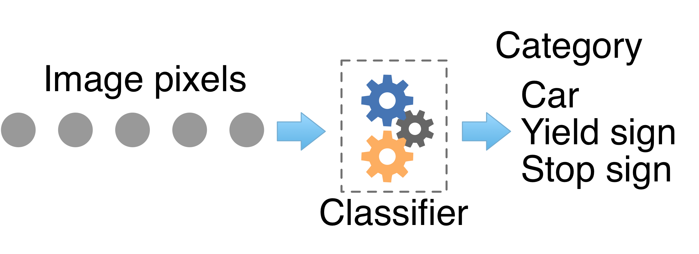
If the target is a numeric value, we're building a predictor (also commonly called a regressor), as shown in Figure 2.5. If the target is a discrete category or class, we're building a classifier (Figure 2.6). We'll learn about classifiers in [foo], but a simple way to think about the difference between predictors and classifiers is illustrated in Figure 2.7 and Figure 2.8. Predictors are usually fitting curves to data and classifiers are drawing decision boundaries in between data points associated with the various categories. There is a tendency to think of predictors and classifiers as totally different problems with different solutions, but they are really the same core problem and most models have both predictor and classifier variants. In fact, the classifier variant is sometimes nothing more than the predictor variant with an additional function that clips, scales, or tweaks the predictor's output.

Machine learning tasks that have both feature vectors x and known targets y fall into the supervised learning category and are the focus of this book. Unsupervised learning tasks involve just x and the target variable is unknown; we say the data is unlabeled. The most common unsupervised task is called clustering that attempts to cluster similar data points together very much like Figure 2.8. In the supervised case, though, we know not only how many categories there are but we also know which records are associated with which category. The goal of clustering is to discover both the number of categories and assign records to categories. As we mentioned in Chapter 1 Welcome!, the vast majority of machine learning problems are supervised and, besides, unsupervised techniques are straightforward to learn after mastering supervised techniques.

Figure 2.9. Distilling model parameters from training data and

A model is a combination of data structure, algorithm, and mathematics that captures the relationship described by a collection of (feature vector, target) pairs. The model records a condensation of the training data in its data structure, which can be anything from the unaltered training set (nearest neighbor model) to a set of decision trees (random forest model) to a handful of weights (linear model). This data structure comprises the parameters of the model and the parameters are computed from the training data. Figure 2.9 illustrates the process.

The process of computing model parameters is called training the model or fitting a model to the data. If a model is unable to capture the relationship between feature vectors and targets, the model is underfitting (assuming there is a relationship to be had). At the other extreme, a model is overfitting if it is too specific to the training data and doesn't generalize well. To generalize means that we get accurate predictions for feature vectors not found in the training set.

Models also have hyper-parameters, which dictate the overall architecture or other aspects of the model. For example, the nearest neighbor model is more specifically called “k-nearest neighbor” because the model finds the nearest k objects then averages their target values to make a prediction. k is the model's hyper-parameter. In a random forest, the number of trees in the forest is the most common hyper-parameter. In a neural network, hyper-parameters typically include the number of layers and number of neurons. Hyper-parameters are specified by the programmer, not computed from the training data, and are often used to tune a model to improve accuracy for a particular data set.

To test generality, we either need to be given a validation set as well as a training set, or we need to split the provided single data set into a training set and a validation set. The model is exposed only to the training set, reserving the validation set for measuring generality and tuning the model. (Later we'll discuss a test set that is used as a final test of generality; the test set is never used while training or tuning the model.) The validation set has both feature vectors and targets and so we can compare the model's prediction with the known correct targets to compute an accuracy metric.

That's a lot to take in, but it will crystallize more and more as we work through more examples. In the next chapter, we'll see how easy it is to train random forest models on some interesting and real data sets.